Fifth Example - 13 Task Network

Figure 1: The resulting cost-time curve

Read on to see how the Time-Cost Curve chart above is produced using the #TimeCostProblemSolved program.

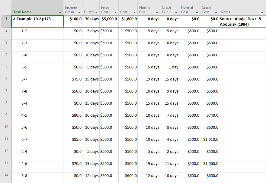
Figure 2: Setup the schedule for producing the time-cost curve. Note that the Fixed Cost for the summary activity is -$5,000 which represents the mathematics of the overhead cost if the project duration was zero. This, together with the incremental cost of $100 per day gives the indirect cost curve (straight line).

Figure 3: Normal schedule

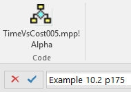
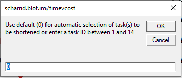
Click the code button, and select default (0) to run the program to compress schedule to 69 days. Repeat again selecting default to compress schedule to 68 days (least-cost schedule). Then select ID 9 followed by ID 13, repeat again two more times, to compress schedule to 65 days. Then select ID 6 followed by ID 11, repeat again three more times to compress schedule to 61 days (least-time schedule).

Figure 4: Fully compressed schedule, represented on the Cost-Time Curve below as the least-time data point (ie 61 days, $8,890).

Figure 5: Cost-Time Curve showing the least-cost schedule would be 68 days, costing $8,500 and the least-time schedule would be 61 days, costing $8,890. #TimeCostProblemSolved